Strawberry Yield Prediction Using Classical Time Series Forecasting Techniques

This project serves to develop a working time series model that can accurately predict strawberry yield for the purpose of improving agricultural productivity.

About Me

Dylan Baxter

Electrical Engineering

I am an second year transfer to Cal Poly’s electrical engineering department.  My interests are currently centered around computer vision, AI, optics, and sensors. I’m always looking to learn new skills, and I like to do photography when my schedule allows.

Acknowledgements

This project was made possible through information made public by the California Strawberry Commission and the NOAA, and by professor Jane Zhang,who facilitated and guided all aspects of the project as advisor.

Strawberry Yield Prediction Using Classical Time Series Forecasting Techniques

Background

Due to its unique climate, scientific advancement and techniques in farm management, the California coast’s strawberry yields have been steadily climbing for decades, and it has come to produce 90% of strawberries in the US . Amidst this industry, advances in robotics, the Internet of things, computer vision, and machine learning are paving the way for advanced harvesting techniques that will reduce waste and allow farmers to allocate resources more precisely.

Currently, specialists are required to provide a yield prediction based on the condition of a small sample of plants, which is inefficient and prone to error. This project acts as an initial step toward the prediction of strawberry yield with past yield data and weather, and establish a foundation for predictions that will incorporate live data collected by IoT systems in the field.

Project Goal

This project aims to create a machine learning model that can successfully predict strawberry yield within 10 trays, 7 days into the future.

Data Characteristics

To train a model for the prediction of strawberry yields in California, we used public yield data published online by the California Strawberry Commission. To extract this data into a processable format, a  dynamic web scraping program was coded in Python to cultivate daily yield data from multiple California districts, dating from 1998 to 2020. Additionally, exogenous weather data in the district of Santa Maria was downloaded from NOAA.gov to aid in yield prediction. For the purpose of testing models, a subset of data from the district of Santa Maria was used, as its yield can be related with more precisely with weather data.

Full dataset from California Strawberry Commission
NOAA Santa Maria weather data from 1999 to 2020

As seen in the yield data shown above, there are several apparent patterns in the data. The first and most obvious is that, due to the seasonal nature of strawberry harvesting, yield data has a strong autocorrelation with lags centered around lag 365.

ACF for Full dataset from California Strawberry Commission

Another key feature of the dataset is the presence of regular downward spikes in yield. This pattern is due to a six day work week, with downward spikes typically representing Sundays, when most farms do not harvest. This could present a significant issue in a training set, as it does not accurately represent the potential for harvest on those days.

Visible weekly downward spikes

Preprocessing

14 Day Rolling Average

In addition to training a model on raw data, 2 preprocessing methods were used as potential alternatives. Initially, a rolling average with a window of 14 was used to attempt to smooth out high frequency, erratic behavior and emphasize trends. This technique was effective but also significantly lowered peaks in yield, which will likely cause under prediction.

Smoothed data compared to full dataset from California Strawberry Commission

Downward Spike Compensation

A preprocessing technique was also developed to reduce the effects of the downward spikes caused by a 6 day work week while preserving the peaks of the original data. It accomplishes this by replacing points that are lower than both their adjacent neighbors with a linear interpolation of those neighbors.

Spike compensated data compared to full dataset from California Strawberry Commission

Finally, all data was split into a into training and test sets, with the training set comprising the first 80 percent of the data and the test set comprising of the latter 20 percent.

Time Series Model Selection

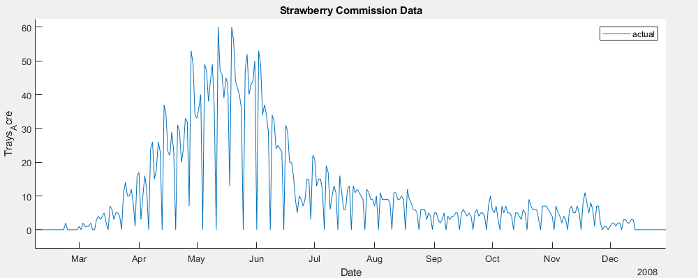
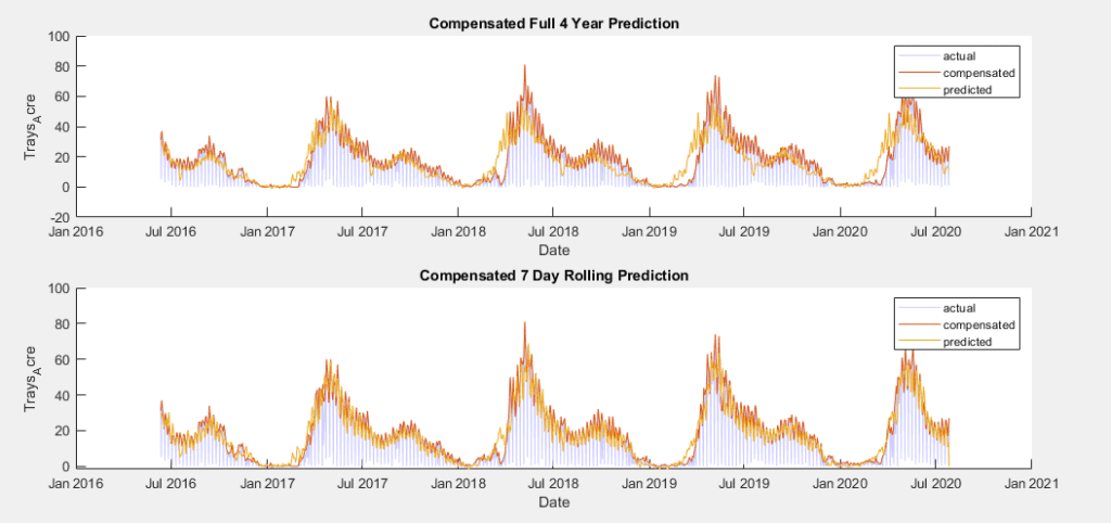
In developing a time series model for this data, the implementation of a SARIMAX model became a clear frontrunner early on, over MLR, EGARCH, GJR and ARIMA models. The seasonal nature of the data allowed for a strong prediction using the previous year’s data, autoregressive terms were able to utilize short term weekly trends, moving average terms predicted based on broader trends, and weather variables could be added as exogenous predictors.

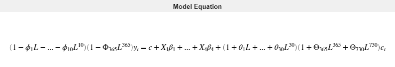
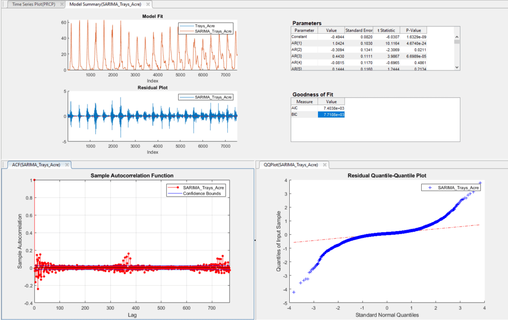
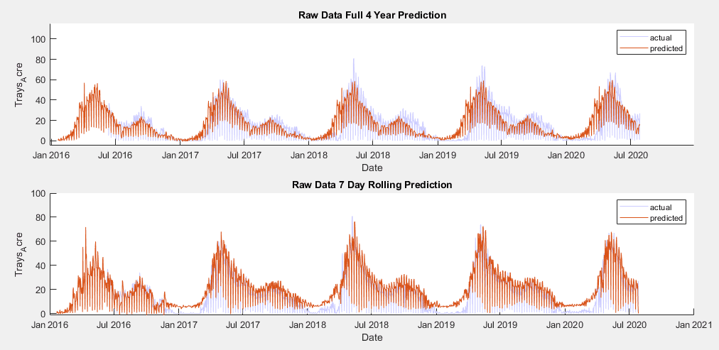
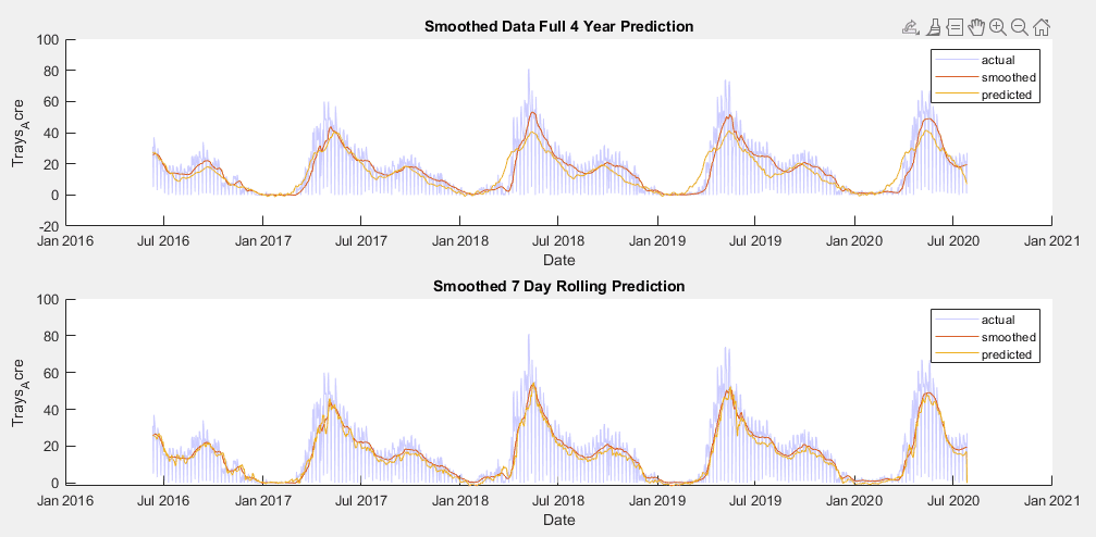
To test for the best possible model, models were trained using the training sets and parameters were raised and lowered individually to determine their effect on the AIC value of the fit. This AIC was then compared across models, with the lowest AIC  values indicating the best fitting.  While increasing any parameter but the integral order generally improved the fit, seasonal autoregressive and moving average orders had the largest effect. The SARIMAX model with the lowest AIC was one with a moving average order of 30(θ terms in model equation), an autoregressive order of 10(ϕ terms), a seasonal moving average order of 2(Θ terms), a seasonal autoregressive order of 1(Φ terms), a seasonal lag of 365, and average temperature, maximum temperature, minimum temperature and precipitation as exogenous predictors(β terms). Three versions of this model have been trained. One for the raw data and two for each of the preprocessed data sets.

AIC Equation
Fit results for yield data training set for SARIMA(10,0,30)(1,0,2)365

Note in the image above that the autocorrelation of the residuals is severely dampened when compared to that of the raw data, and now only show weak autocorrelation near lag 365. This represents a seasonality that is due to extreme spikes in yield at the peak of the harvesting season. These peaks are difficult to model  and cause predictable, yearly increases in yield residuals.

Prediction Results

When put into action, this model performed surprisingly well for prediction of the entire testing set, which emcompasses four years of yield data. However, after one year it’s seasonal components start to use data from previous forecasted values, and the yearly pattern undergoes little change, despite changing ground truth data. To compensate for this, a matlab script was developed to perform a rolling forecast  7 days ahead of known values. This better fit the test set, allowed trends to be more dynamic, and accurately accounted for the information that will be available to farmers for predictions.

4 year and 7 day rolling forecast trained using raw data

AIC Values for Model Trained with Raw Data:

  • 4 Year Prediction: 8.380e+3
  • 7 Day Rolling Prediction:  8.603e+3
The model trained on the raw data performed better than expected, but still suffered from inability to reach extreme spikes in yield, both upward and downward. When smoothed, the training data allowed the model to remain at a constant middle ground between the highs and lows during peak harvesting season. This increased fit marginally from the model trained on the raw data.
4 year and 7 day rolling forecast trained using smoothed data

AIC Values for Model Trained with Smoothed Data:

  • 4 Year Prediction: 7.024e+3
  • 7 Day Rolling Prediction: 6.927e+3

Further,  if the model is trained on a dataset where the peaks are preserved, the best possible performance is achieved and the resulting prediction is closest to the true potential yield data. As shown in the figure below, the 4 year

4 year and 7 day rolling forecast trained using spike compensated data

AIC Values for Model Trained with Spike Compensated Data:

  • 4 Year Prediction: 7.245e+3
  • 7 Day Rolling Prediction: 4.9807e+3

Conclusions and Future Work

The results of this project indicate the most effective time series model for the prediction of Strawberry yield is  a SARIMAX(10,0,30)(1,0,2)365 model using daily maximum temperature, minimum temperature and average temperature, precipitation as exogenous predictors and trained with yield data that is compensated for downward spikes, and forecasted with a 7 day rolling forecast. Unfortunately, this model does not meet the desired goal established at the beginning of the project, but it does provide predictions within tolerance for a majority of the yearly cycle, and represents a solid proof of concept of  utilizing  machine learning for strawberry yield prediction.

Residuals of the 7 day rolling forecast trained using spike compensated data

In order to to overcome the erratic spikes in yield that occur during peak harvesting season, neural networks and other machine learning algorithms should be explored as potential options for modeling strawberry yield.  In addition, we intend to extend the rolling forecast range to 14 days, and incorporate strawberry life cycle data from IoT camera and computer vision systems.

Share

Share on facebook
Share on twitter
Share on linkedin

Coronavirus Update and Resources