Student Researcher

Shea Charkowsky
MECHANICAL ENGINEERING
Shea is a third-year student from Santa Clara, CA. Over the course of the summer, he developed and implemented several improvements on the previous MATLAB model of the Gold Tree Solar Array, including a full redesign of the code’s shade calculation algorithm.
He enjoys problem-solving and creativity of all kinds, from brain puzzles and mathematics to hip-hop dance and piano.
Acknowledgements
My thanks go to REC Solar for sponsoring this project, to Dr. Andrew Davol, Dr. Jacques Belanger, and Andy Kim for building the foundation for this work, and to Dr. Davol and Dr. Belanger for their guidance and support.
MATLAB Model of the Gold Tree Solar Array
The Issue of
Interrow Shading
Interrow shading can cause significant power loss for solar arrays, since even one low-generating cell limits current through the rest. In other words, an entire panel subsection can be shut down by one blocked cell.
Sun-tracking arrays can avoid this by backtracking, tilting panels upward just enough to prevent such shading. However, Cal Poly’s Gold Tree Solar Array is on such uneven terrain that eliminating all shading via backtracking would sacrifice power in a different way—from indirectness of sunlight. A balance must be struck between these two opposing issues that minimizes their effects and maximizes power output.
Our Goal
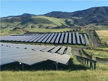
Our overarching objective is to construct a MATLAB model of the Gold Tree Solar Array as a fast and convenient tool for testing different tracking parameters for eventual power optimization.
The version existing at the summer’s start required impractical runtimes and did not incorporate any empirically obtained environmental data. Our goal this summer was to add representative climate and sunlight data to the model and to develop a faster calculation of shade shape. Completing these tasks would be among the final steps required before beginning parameter tests and optimization.
–
These two panels are directly tracking the sun; the gold sunlight vector aligns with the blue panel direction vector. In this case, doing so causes interrow shading of the panel on the right.
An Explanation of Backtracking
In the morning and evening, the sun is low enough that direct tracking causes interrow shading. However, panels can be tilted upward and out of each other’s way to avoid this shade. Doing so is called backtracking.
Though backtracking can remove interrow shading, it reduces the panels’ efficiency since they don’t directly face the sun. Thus, backtracking too early or too late both yield suboptimal power from the solar array. Our goal is to find the compromise between these that achieves maximum power output.
These panels are backtracking; note that the panel direction vector does not align with the sunlight vector. Interrow shading has been avoided, but the panels now receive less power per area.
–
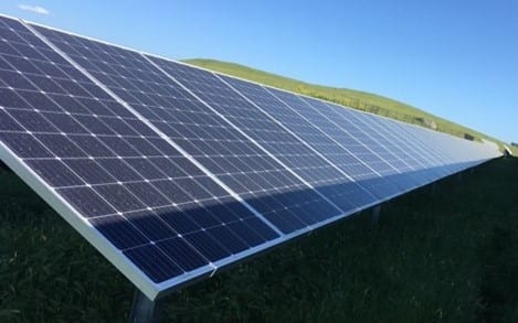
Significant interrow shading on one of the Gold Tree array’s panels, occurring around 5 PM on April 23, 2020.
Improvements on the Previous MATLAB Model
Three main changes to the model fulfilled our goals for the summer: adding temperature data representing San Luis Obispo’s climate, incorporating sunlight levels measured on-site in 2019, and designing a new method of calculating shade boundaries. We also created a SolidWorks model to verify the MATLAB model’s accuracy.
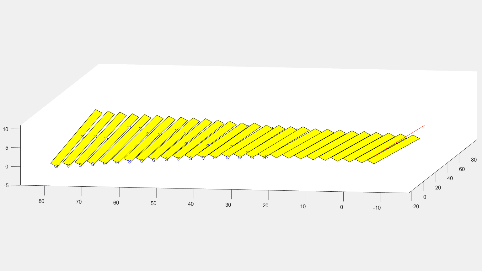
A visualization of the MATLAB model’s panels and shade boundaries, the corners of which are marked with blue circles.
Solar Irradiance Data
The previous model’s calculations assumed full sun, but a more realistic model would account for cloudiness. To do this, we needed empirical data on sunlight strength.
Solar irradiance is the rate per area at which a surface receives or would receive solar energy. If you were to hold a panel straight at the sun, you would measure direct normal irradiance (DNI), an indicator of overall sunlight strength. If you tilted it at an angle, you would intercept the panel’s smaller plane-of-array (POA) irradiance, as shown in the figure below. If we call the incident angle a, then
DNI cos(a) = POA.
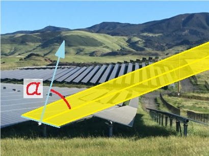
Since the panel above doesn’t directly face the sun, only a portion of the possible power from DNI is captured as POA irradiance.
We needed representative DNI data for a complete year, but we had only panel tilt angles and measured POA irradiance. To obtain DNI values, we wrote a function that fetches this POA data, calculates the incident angle, and solves the equation above for DNI.
Further Detail on Angle Calculation
Finding the sun’s incident angle involved several components. For a given date and time, we needed both the unit vector Vs pointing toward the sun and the unit vector Vp normal to the panel. With these, we could find the cosine of the incident angle using the dot product, since
Vs • Vp = |Vs| |Vp| cos(a) = cos(a).
A function from PVLIB, an open-source collection of photovoltaic modeling software, provided solar zenith and azimuth angles, which we converted to Cartesian to find Vs. Assuming horizontal and north-south oriented panels enabled simple trigonometry to define Vp. The dot product of these yielded the cosine of the incident angle by which POA was divided in order to find DNI.
Shade Shape by Projection and Coordinate Change
In a mathematical sense, shade is a projection parallel to sunlight of one object’s shape onto another. To find shade boundaries in our case, we needed only to determine the projection of each panel’s edges onto the next, a much easier calculation for MATLAB than the previous method of mathematical raytracing.
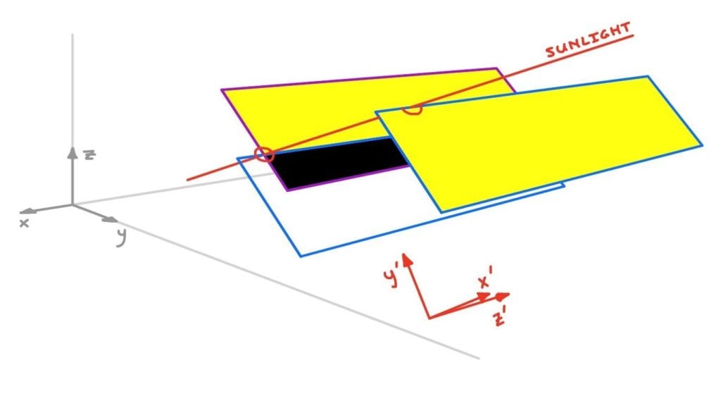
Above, the blue panel casts a shadow onto the purple panel behind it. The projected edges of the blue panel define the purple panel’s shaded region.
The MATLAB model’s power output function receives each shaded region’s two upper corners, an example of which is the full red circle in the figure above. Note, however, that this point does not correspond to any panel corners, real or projected. We must therefore determine the intersection of the front panel’s projected edges with the rear panel’s true edges.
In 3D global coordinates, this task quickly escalates into unwieldy vector operations and shading cases. However, enormous simplification is achieved by nothing more than a change of perspective.
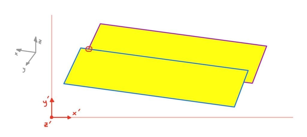
From the sun’s point of view, the intersections between the two panels’ edges are easy to see—and to calculate.
The task becomes much easier after the coordinate trans- formation depicted in red in the images above, which establishes a system having its z’-axis pointed toward the sun. Since looking down the z’-axis is the same as looking in the direction of sunlight, real and projected edges coincide in the x’y’-plane.
Each intersection is then readily found in 2D, followed by the z’-coordinate that places it on the appropriate panel. Transforming twice more yields shade coordinates relative to the panel, and these feed directly into the power output function.
SolidWorks Model
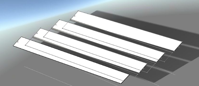
SolidWorks’ built-in solar lighting is rendered on four Gold Tree panels. The grey transparent rectangles are projected shade.
The Solidworks model of four panels shown above was created to verify the shade dimensions measured on site and calculated in the MATLAB model. Panels were first positioned according to surveyed coordinates, and then each panel surface was projected along the direction of sunlight onto the next panel to simulate shade, whose boundaries could then be manually measured.
All three methods produced similar shade dimensions, giving us further confidence in the MATLAB model.
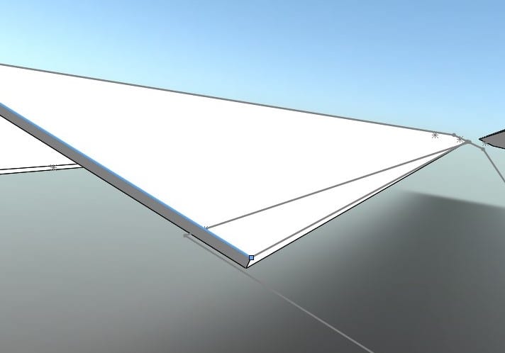
The same panel at the same date and time as shown in the image just before “Improvements on the Previous MATLAB Model.”
Air Temperature Data
A solar cell’s efficiency depends on its surface temperature, but we were unable to measure this since the cell temperature sensor had stopped working. Instead, cell temperature was estimated from ambient air temperature and solar irradiance according to Kim (2020).
Meteorological data provided representative hourly air temperature values, and a function was written to store, retrieve, and interpolate to the quarter-hour these values for use by the MATLAB model.
–
Results
Our main concern was whether the new version of the MATLAB model could produce reasonable outputs faster. Based on tests on a personal laptop, the former raytracing program would have taken an estimated 1.5 hours to analyze power from all 27 modeled panels for the full day of April 23, 2020. The same task was completed by the new projection version in less than 30 seconds. Since speed is crucial for iterative testing, this result greatly benefits our overarching objectives.
Future Work
Though the ultimate goal for the MATLAB model is tracking parameter optimization, a few steps must be completed first.
The model should undergo more rigorous accuracy tests, including statistical analysis comparing its output to that of the Gold Tree site. This may include tests over longer time intervals (e.g. over a full month) to compare averages. Additionally, we modeled only one of the twelve zones of the Gold Tree array; modeling the other eleven zones would then enable us to run tests on the entire site for any time period.
This project was sponsored by


